In this series of articles I will explain the inner workings of a neural network. I will lay the foundation for the theory behind it as well as show how a competent neural network can be written in few and easy to understand lines of Java code.

This is the first part in a series of articles:

• Part 1 – Foundation. (This article)
• Part 2 – Gradient descent and backpropagation.
• Part 3 – Implementation in Java.
• Part 4 – Better, faster, stronger.
• Part 5 – Training the network to read handwritten digits.
• Extra 1 – Data augmentation.
• Extra 2 – A MNIST playground.

Background

Some weeks ago I decided to pick up on machine learning. Most of all my interest is Applied machine learning and the business opportunities and new software this paradigm might bring. I figured that a reasonable way forward then would be to pick up any framework such as TensorFlow or DL4J and start playing around. So I did … and became frustrated. The reason is that just setting up a good behaving neural network in any of these frameworks requires a fair amount of understanding of the concepts and the inner workings: Activation functions, Optimizers, Regularization, Drop-outs, Learning-rate-annealing, etc. – I was clearly groping in the dark.

I just had to get some deeper understanding of it all. Consequently I dived head first into the vast internet-ocean of information and after a week of reading I unfortunately realized that not much of the information had turned into knowledge. I had to rethink.

Long story short: I decided to build a minor neural network myself. As a get-the-knowledge-I-need-playground.

It turned out fine. The practical/theoretical mix required when building from scratch was just the right way for me to get a deeper understanding. This is what I’ve learned.

Neural networks

From outside a neural network is just a function. As such it can take an input and produce an output. This function is highly parameterized and that is of fundamental importance.

Some of those parameters we set ourselves. Those parameters are called hyper-parameters and can be seen as configuration of our neural network. The majority of parameters however are inherent to the network and nothing we directly control. To understand why those are important we need to take a look at the inside.

A simple neural network typically consists of a set of hidden layers each containing a number of neurons, marked yellow in the picture. The input layer is marked blue.

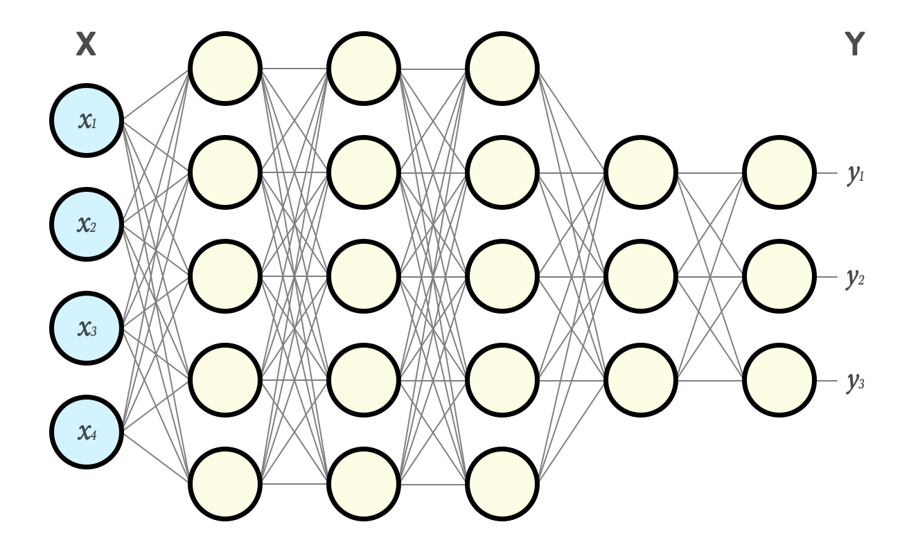
In the configuration above the input is a vector X of size 4 and output is a vector Y of size 3.

As you can see in the picture there is a connection between every neuron in one layer to every neuron in the next¹. Every such connection is in fact a parameter or weight. In this example we already have 94 extra parameters in form of weights. In bigger networks there can be magnitudes more. Those weights will define how the network behaves and how capable it is to transform input to a desired output.

The neuron

Before I explain how the network as a whole can be used to transform data we need to zoom in further. Say hello to a single neuron:

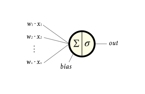
The input to every neuron is the weighted sum of the output from every neuron in the previous layer. In the example this would be:

$$\sum_{i=0}^n w_i \cdot x_i $$

To that we add a scalar value called a bias, b, which gives a total input to the neuron of:

$$z = \left(\sum_{i=0}^n w_i \cdot x_i\right) + b$$

A short side-note: When considering the entire layer of neurons, we instead write this in vector form z = Wx + b, where z, x and b are vectors and W is a matrix².

• x contains all outgoing signals from the preceding layer.
• b contains all biases in the current layer.
• W has all the weight for all connections between preceding layer and the current.

The input signal is then transformed within the neuron by applying something called an activation function, denoted σ. The name, activation function, stems from the fact that this function commonly is designed to let the signal pass through the neuron if the in-signal z is big enough, but limit the output from the neuron if z is not. We can think of this as the neuron firing or being active if stimuli is strong enough.

More importantly the activation function adds non-linearity to the network which is important when trying to fit the network efficiently (by fit the network I mean train the network to produce the output we want). Without it the network would just be a linear combination of its input.

Quite often an activation function called Rectified Linear Unit, or ReLU, is used (or variants thereof). The ReLU is simply:

$$
σ(z) = max(z, 0)
$$

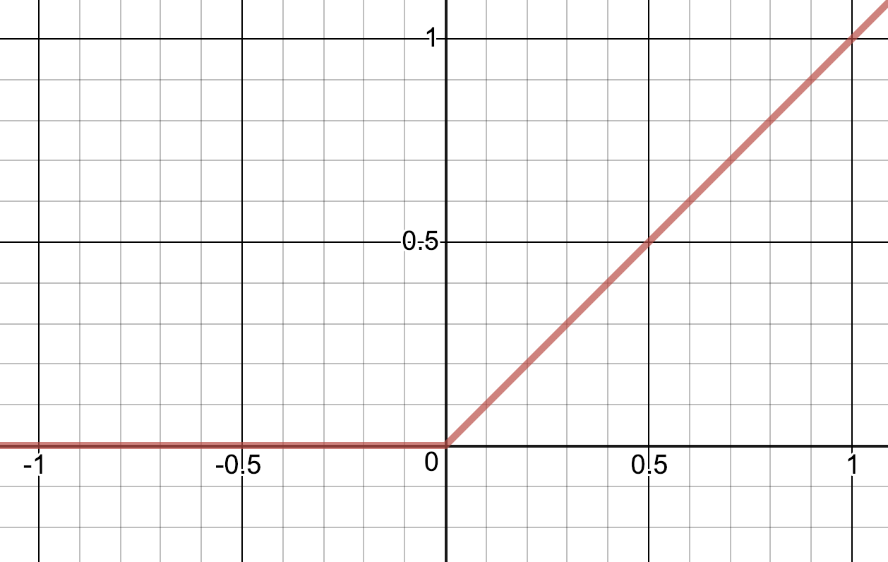
Another common activation function is this logistic function, called the sigmoid-function:

$$
σ(z) ={\frac {1}{1+e^{-z}}}
$$

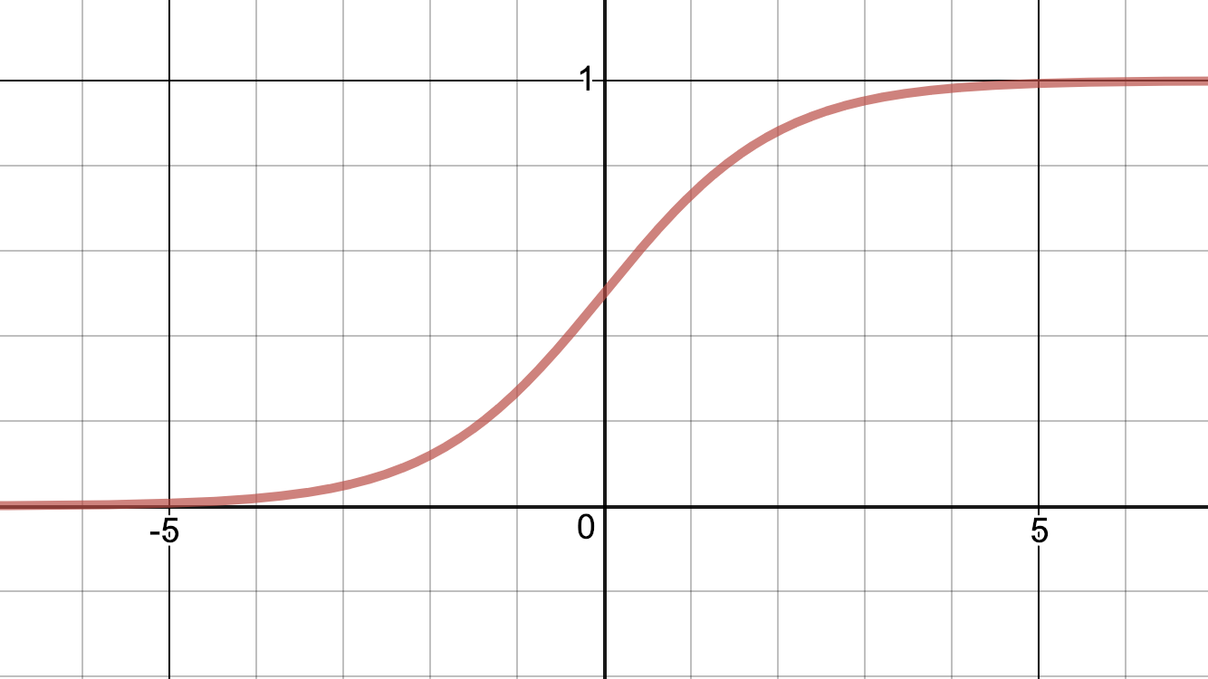
As you can see from the graphs they both behave the way I described: They let the signal pass if big enough, and limits it if not. 

Finally, after having applied the activation function to z, getting σ(z), we have the output from the neuron.

Or stated in vector-form: after having applied the activation function to vector z, getting σ(z) (where the function is applied to every element in the vector z) we have the output from all the neurons in that layer.

Feed forward

Now we have all the bits and pieces to describe how to apply the entire neural network (i.e. “the function”) to some data x to get an output y = f(x).

We simply feed the data through every layer in the network. This is called feed forward and it works like this:

• Input x and start in the first hidden layer:
  • For every neuron in the current layer n, take the weighted sum of the output from every connected neuron in the preceding layer n – 1. Add the bias and apply the activation function.
  • Proceed to layer n + 1 but now use the output values from layer n as input.
• Now carry on layer by layer until you reach the last layer. The output from those neurons will give y.

Let’s look at a simple example:

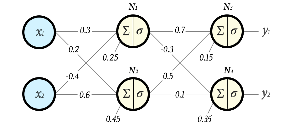
Assume that we have chosen the sigmoid function as activation in all layers:

$$σ(z) = {\frac {1}{1+e^{-z}}}$$

Now let us, layer by layer, neuron by neuron, calculate what output y this network would give on the input vector x = [2  3].

N1 = σ(0.3 · 2 + (-0.4) · 3 + 0.25) = σ(-0.35) = 0.41338242108267
N2 = σ(0.2 · 2 + 0.6 · 3 + 0.45) = σ(2.65) = 0.934010990508781
N3 = σ(0.7 · N1 + 0.5 · N2 + 0.15) = σ(0.90637319001226) = 0.712257432295742
N4 = σ((-0.3) · N1 + (-0.1) · N2 + 0.35) = σ(0.132584174624321) = 0.533097573871501

Hence, this network produces the output
y = [0.7122574322957417  0.5330975738715015]
on the input x = [2  3].

If we are lucky, or skilled at setting initial weights and biases, this might be exactly the output we want for that input. More likely it is not at all what we want. If the latter is the case we can adjust the weights and biases until we get the output we want.

Let’s for a while think about why a neural network is designed the way it is and why adjustments of weights and biases might be all that is needed to make the network behave more to our expectations.

The expressiveness of a neural network

The high parameterization of the network makes it very capable of mimicking almost any function. If the function we try to mimic is more complex than what is possible to express by the set of weights and biases we can just create a slightly larger network (deeper and/or wider) which will give us more parameters which in turn would be better to fit the network to the function we want.

Also note that by the way a neural network is constructed we are free to chose any dimension on the input and any dimension on the output. Often neural networks are designed to reduce dimensions –  i.e. map points from a high dimensional space to points in a low dimensional space. This is typical for classification of data. I will get back to that with an example in the end of this article.

Now consider what happens in each neuron: σ(Wx + b) – i.e. we feed the activation function the signal from the preceding layer but we scale and translate it first. So, what does it mean to scale and translate an argument to a function? Think about it for a while.

For simplicity, let’s see what happens i two dimensions when we scale the input to a function.

Here is what the sigmoid-function looks like with a non-scaled input, i.e. σ(x):

And here is what it looks like if we scale the input by a factor 5, i.e. σ(5x). As you can see, and probably have guessed, scaling the input compresses or expands the function over the x-axis.

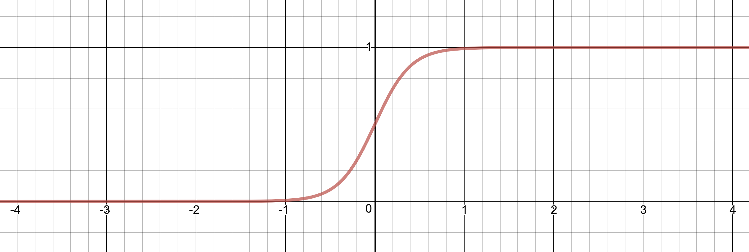
Finally, adding a scalar to the input means we move the function on the x-axis. Here is σ(5x – 4):

So by scaling and translating the input to the activation function we can move it and stretch it.

Also remember that the output from one layer is the input to the next. That is, a curve (such as any of the ones above) produced in layer L will be scaled and translated before fed to the activation function in layer L+1. So now we need to ask, what does it mean to scale and translate the output from a function in layer L? Scaling simply means altering the magnitude of that signal, i.e. stretch or compress it along the y-axis. Translating obviously mean moving it along the y-axis.

So what does this give us?

Although the discussion above does not prove anything it strongly suggest that by altering weights and biases of a neural network we can stretch and translate input values (the individual vector components even) in a non-linear way pretty much to our liking.

Also consider that the depth of a network will let weights operate on different scales and with different contributions to the total function – i.e. an early weight alters the total function in broad strokes, while a weight just before the output layer operate on a more detailed level.

This gives the neural network a very high expressiveness but at the cost of having heaps of parameters to tune. Fortunately we do not have to tune this by hand. We can let the network self-adjust so that the output better meet our expectations. This is done via a process called gradient descent and backpropagation which is the topic of the next article in this series, Part 2 – Gradient descent and backpropagation.

Now, how can a function act intelligently?

We have concluded that a neural network can mimic a mapping (a function) from a vector x to another vector y. At this point it is fair to ask: In what way does this help us?

One quite common way of using a neural network is to classify data it has never seen before. So, before wrapping up this already lengthy article, I will give a glimpse about a practical example of classification. An example that we will get back to in later articles.

When writing a neural network one of the first task typically thrown at it is classification of hand written digits (kind of the “Hello World” in machine learning). For this task there is a dataset of 60 000 images of hand written digits called the MNIST dataset. The resolution is 28 x 28 and the color in each pixel is a greyscale value between 0 and 255. The dataset is labeled which means that it is specified what number each image represent.

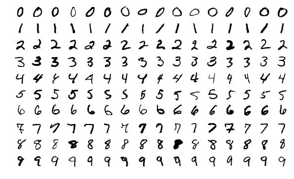
If we flatten out each image – i.e. take each row of the image and put it in a long line – we will get a vector of size 28 x 28 = 784. Also we normalize the greyscale values to range between 0 and 1. Now it would be nice if we could feed this vector x to a neural network and as an output get a y-vector of size 10 telling what number the network thinks the input represent (i.e. each element of the output vector telling what probability the network gives the image being a zero, a one, a two, … , a nine). Since the MNIST dataset is labeled we can train this network which essentially means: auto-adjust the weights and biases. The cool thing is that if that training is done right the network will be able to classify images of hand written digits it has never seen before – something that would have been very hard to program declaratively.

How could this be?

I will try to explain that with a concluding food for thought: Each input vector x can be seen as a single point in a 784-dimensional space. Think about it. A vector of length 3 represents a point in 3D. A vector of length 784 then represents a point in 784D. Since each pixel value is normalized between 0 and 1 we know that all points for this dataset lays within the unit cube, i.e. between 0 and 1 on all 784 axes. It is reasonable to think that all points representing a number N lay fairly close to each other in this space. For instance all images of the digit 2 will lay close to each other in some subspace, as well as all 7:s will be close but in a different subspace. When designing this network we decided that the output should be a vector of size 10 where each component is a probability. This means the output is a point in a 10-dimensional unit cube. Our neural network maps points in the 728D-cube to points in the 10D-cube.

Now, what fitting the network in this particular case really means is finding those subspaces in the 784D-input space with our neural network function and transform (scale, translate) them in such a way that they are clearly separable in 10D. For instance: We want all inputs of the digit seven, however they may differ slightly, to output a vector y where the component representing the number seven is close to 1 and all other 9 components are close to 0.

I tend to think of the fitting process as shrink wrapping surfaces (hyperplanes) around those subspaces³. If we do not shrink wrap those surfaces too hard (which would result in something called over-fitting) it is quite likely that digits that the network has not yet seen still would end up within the correct subspace – in other words, the network would then be able to say: “Well, I have never seen this digit before but it is within the subspace which I consider to be number 7”.

And that is somewhat cool!

Ok, that will do for an intro. Feedback is welcome!

Now, onto next article in this series were you will learn how neural networks can be trained: Part 2 – Gradient descent and backpropagation.

This article has also been published in the Medium-publication Towards Data Science. If you liked what you’ve just read please head over to the medium-article and give it a few Claps. It will help others finding it too. And of course I hope you spread the word in any other way you see fit. Thanks!

Footnotes:

1. This article describes a dense feed forward network – a multilayer perceptron. That network design was chosen for its simplicity and accessibility. It is good to know however that there are lots of different networks which all of them are suitable for different types of tasks.
2. So you might wonder how it is possible to write the whole layer operation in that short vector notation? If you recall how multiplying a matrix with a vector works you will realize that when doing Wx you actually do a weighted summation of the x-vector over and over (per row in the W-matrix) resulting in a vector. Adding the b-vector to that will give z.
3. Strictly speaking this is not what happens. But I find it to be a helpful mental image.