Part 5 – Training the network to read handwritten digits

In this final article we will see what this neural network implementation is capable of. We will throw one of the most common dataset at it (MNIST) and see if we can train a neural network to recognize handwritten digits.

This is the fifth and last part in this series of articles:

The MNIST dataset

The MNIST database contains handwritten digits and has a training set of 60.000 samples, and a test set of 10.000 samples. The digits are centered in a fixed-size image of 28×28 pixels.

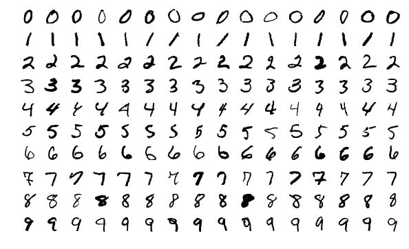
This dataset is super convenient for anyone who just wants to explore their machine learning implementation. It requires minimal efforts on preprocessing and formatting.

Code

All code for this little experiment is available here. This project is of course dependent on the neural network implementation too.

Reading the datasets in java is straightforward. The data format is described on the MNIST pages.

Each digit is stored in a class called DigitData. That class of course contains the data (i.e. the input) and the label (i.e. the expectation). I also added a small trick to enhance the toString() of theDigitData class:

/**
 * Simply converts gray-scale to an ascii-shade
 */
private char toChar(double val) {
    return " .:-=+*#%@".charAt(min((int) (val * 10), 9));
}

/**

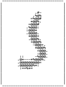
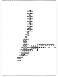
* Simply converts gray-scale to an ascii-shade

private char toChar(double val) {

return " .:-=+*#%@".charAt(min((int) (val * 10), 9));

}

Calling toString() actually gives an ascii-shaded output of the data:

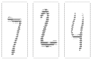
This has been convenient when examining which digits the network confuses for other digits. We will get back to that in the end of this article.

Network setup

The boundary layers are given by our data:

The input layer takes every pixel of the image as input and has to be of size 28 x 28 = 784.
The output layer is a classification – a digit between 0 and 9 – i.e. size 10.

The hidden layers requires more exploring and testing. I tried a few different network layouts and realized that it was not that hard to get good accuracy with a monstrous net. As a consequence I decided to keep the number of hidden neurons down just to see whether I still could get decent results. I figure that a constrained setup would teach more about how to get that extra percentage of accuracy. I decided to set the max hidden neurons to 50 and started exploring what I could attain.

I had quite good result early on with a funnel-like structure with only 2 hidden layers and kept on exploring that. For instance the first one with 36 and the second with 14 neurons.

784 input ⇒ 36 hidden ⇒ 14 hidden ⇒ 10 output neurons

After some trial and error I decided to use two activation functions which has not been presented in previous articles in this series. The Leaky ReLU and the Softmax.

Leaky ReLU is a variant of ReLU. Only difference is that it is not totally flat for negative inputs. Instead it has a small positive gradient.

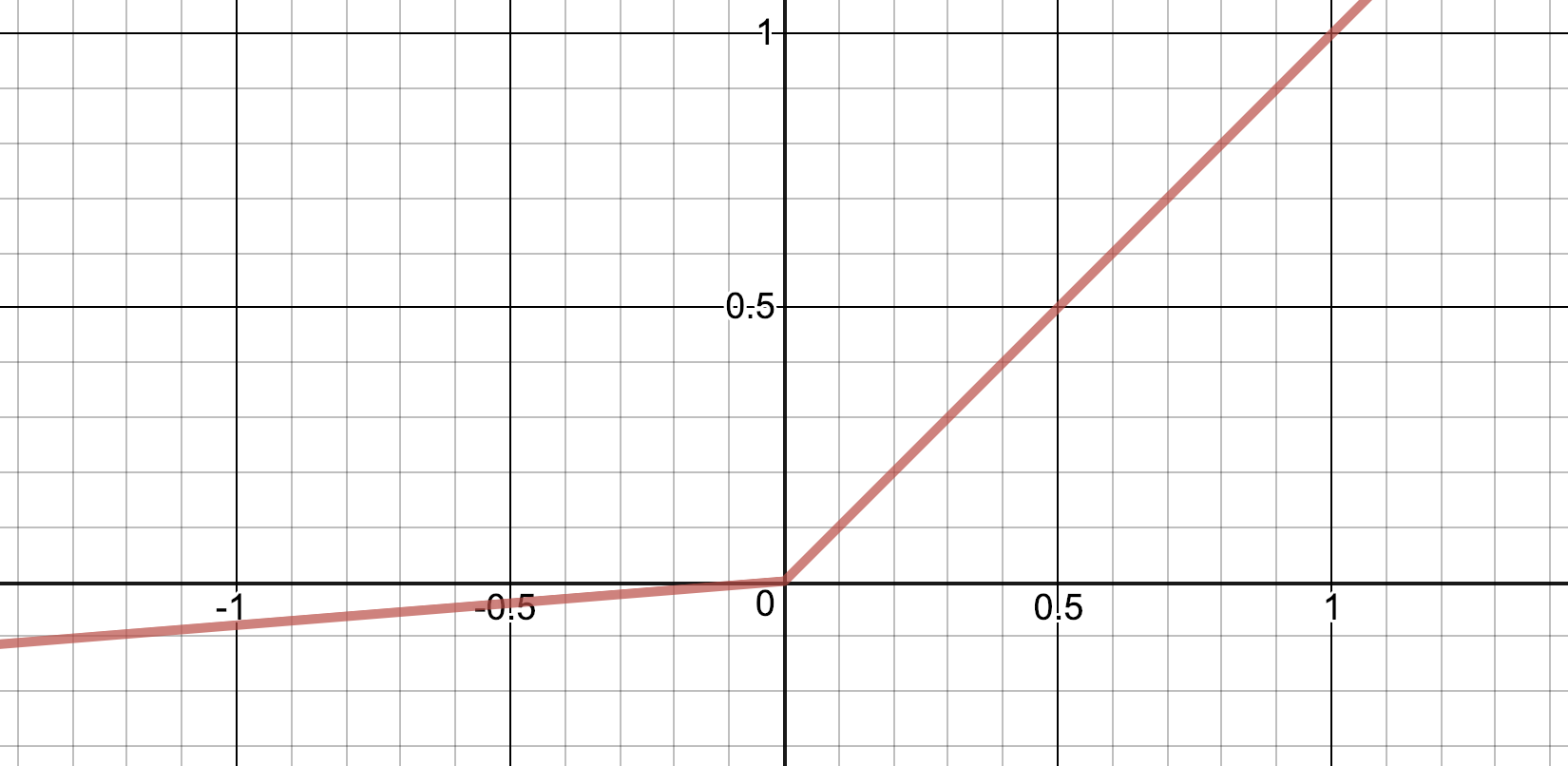
They were initially designed to work around the problem that the zero-gradient part of ReLU might shut down neurons. Also see this question on Quora for details on when and why you might want to test Leaky ReLU instead of ReLU.

Softmax is an activation function which you typically use in the output layer when you do classification. The nice thing with softmax is that gives you a categorical probability distribution – It will tell you the probability per each class in the output layer. So, suppose we did send the digit data representing the digit 7 through the network it might output something like:

Class	P
0	0.002
1	0.011
2	0.012
3	0.002
4	0.001
5	0.001
6	0.002
7	0.963
8	0.001
9	0.005
	Σ = 1.0

As you can see the probability is highest for digit 7. Also note that the probabilities sum to 1.

Softmax can also of course be used with a threshold so that if neither of the classes get a probability above that threshold we can say that the network did not recognize anything in the input data.

The bad thing about Softmax is that it is not as simple as other activation functions. It gets a bit uglier both in the forward and backpropagation pass. It actually broke my activation abstraction where I until the introduction of softmax could define an Activation as only the function itself for forward pass, fn(), and the derivative step of that function for backpropagation, dFn().

The reason Softmax did this is that its dFn() (\(\frac{\partial o}{\partial i}\)) can utilize the last factor from the chain rule (\(\frac{\partial C}{\partial o}\)) to make the calculation clearer/easier. Hence the Activation abstraction had to be extended to deal with calculating the \(\frac{\partial C}{\partial i}\) product.

In all other activation functions this is simply a multiplication:

// Also when calculating the Error change rate in terms of the input (dCdI)
// it is just a matter of multiplying, i.e. ∂C/∂I = ∂C/∂O * ∂O/∂I.
public Vec dCdI(Vec out, Vec dCdO) {
    return dCdO.elementProduct(dFn(out));
}

// Also when calculating the Error change rate in terms of the input (dCdI)

// it is just a matter of multiplying, i.e. ∂C/∂I = ∂C/∂O * ∂O/∂I.

public Vec dCdI(Vec out, Vec dCdO) {

return dCdO.elementProduct(dFn(out));

}

But in softmax it looks like this (see dCdI()-function below):

// --------------------------------------------------------------------------
// Softmax needs a little extra love since element output depends on more
// than one component of the vector. Simple element mapping will not suffice.
// --------------------------------------------------------------------------
public static Activation Softmax = new Activation("Softmax") {
    @Override
    public Vec fn(Vec in) {
        double[] data = in.getData();
        double sum = 0;
        double max = in.max();    // Trick: translate the input by largest element to avoid overflow.
        for (double a : data)
            sum += exp(a - max);

        double finalSum = sum;
        return in.map(a -> exp(a - max) / finalSum);
    }

    @Override
    public Vec dCdI(Vec out, Vec dCdO) {
        double x = out.elementProduct(dCdO).sumElements();
        Vec sub = dCdO.sub(x);
        return out.elementProduct(sub);
    }
};

// --------------------------------------------------------------------------

// Softmax needs a little extra love since element output depends on more

// than one component of the vector. Simple element mapping will not suffice.

// --------------------------------------------------------------------------

public static Activation Softmax = new Activation("Softmax") {

@Override

public Vec fn(Vec in) {

double[] data = in.getData();

double sum = 0;

double max = in.max(); // Trick: translate the input by largest element to avoid overflow.

for (double a : data)

sum += exp(a - max);

double finalSum = sum;

return in.map(a -> exp(a - max) / finalSum);

}

@Override

public Vec dCdI(Vec out, Vec dCdO) {

double x = out.elementProduct(dCdO).sumElements();

Vec sub = dCdO.sub(x);

return out.elementProduct(sub);

}

};

So, all in all my setup typically is:

NeuralNetwork network =
        new NeuralNetwork.Builder(28 * 28)
                .addLayer(new Layer(36, Leaky_ReLU))
                .addLayer(new Layer(14, Leaky_ReLU))
                .addLayer(new Layer(10, Softmax))
                .initWeights(new Initializer.XavierNormal())
                .setCostFunction(new CostFunction.Quadratic())
                .setOptimizer(new Nesterov(0.02, 0.87))
                .l2(0.00010)
                .create();

NeuralNetwork network =

new NeuralNetwork.Builder(28 * 28)

.addLayer(new Layer(36, Leaky_ReLU))

.addLayer(new Layer(14, Leaky_ReLU))

.addLayer(new Layer(10, Softmax))

.initWeights(new Initializer.XavierNormal())

.setCostFunction(new CostFunction.Quadratic())

.setOptimizer(new Nesterov(0.02, 0.87))

.l2(0.00010)

.create();

With that in place, let’s start training!

Training loop

The training loop is simple.

I shuffle the training data before each epoch (an Epoch is what we call a complete training round of all available training data, in our case 60.000 digits) and feed it through the network with training flag set to true.
After every 5:th epoch I also run the test data through the network and log the results but do not train the network while doing so.

The code looks like this:

List<DigitData> trainData = FileUtil.loadImageData("train");
List<DigitData> testData = FileUtil.loadImageData("t10k");

int epoch = 0;
double errorRateOnTrainDS;
double errorRateOnTestDS;

StopEvaluator evaluator = new StopEvaluator(network, 10, null);
boolean shouldStop = false;

long t0 = currentTimeMillis();
do {
    epoch++;
    shuffle(trainData, getRnd());

    int correctTrainDS = applyDataToNet(trainData, network, true);
    errorRateOnTrainDS = 100 - (100.0 * correctTrainDS / trainData.size());

    if (epoch % 5 == 0) {
        int correctOnTestDS = applyDataToNet(testData, network, false);
        errorRateOnTestDS = 100 - (100.0 * correctOnTestDS / testData.size());
        shouldStop = evaluator.stop(errorRateOnTestDS);
        double epocsPerMinute = epoch * 60000.0 / (currentTimeMillis() - t0);
        log.info(format("Epoch: %3d    |   Train error rate: %6.3f %%    |   Test error rate: %5.2f %%   |   Epocs/min: %5.2f", epoch, errorRateOnTrainDS, errorRateOnTestDS, epocsPerMinute));
    } else {
        log.info(format("Epoch: %3d    |   Train error rate: %6.3f %%    |", epoch, errorRateOnTrainDS));
    }

} while (!shouldStop);

List<DigitData> trainData = FileUtil.loadImageData("train");

List<DigitData> testData = FileUtil.loadImageData("t10k");

int epoch = 0;

double errorRateOnTrainDS;

double errorRateOnTestDS;

StopEvaluator evaluator = new StopEvaluator(network, 10, null);

boolean shouldStop = false;

long t0 = currentTimeMillis();

do {

epoch++;

shuffle(trainData, getRnd());

int correctTrainDS = applyDataToNet(trainData, network, true);

errorRateOnTrainDS = 100 - (100.0 * correctTrainDS / trainData.size());

if (epoch % 5 == 0) {

int correctOnTestDS = applyDataToNet(testData, network, false);

errorRateOnTestDS = 100 - (100.0 * correctOnTestDS / testData.size());

shouldStop = evaluator.stop(errorRateOnTestDS);

double epocsPerMinute = epoch * 60000.0 / (currentTimeMillis() - t0);

log.info(format("Epoch: %3d | Train error rate: %6.3f %% | Test error rate: %5.2f %% | Epocs/min: %5.2f", epoch, errorRateOnTrainDS, errorRateOnTestDS, epocsPerMinute));

} else {

log.info(format("Epoch: %3d | Train error rate: %6.3f %% |", epoch, errorRateOnTrainDS));

}

} while (!shouldStop);

And the running through the entire dataset is done in batches and in parallel (as already shown in last article):

/**
 * Run the entire dataset <code>data</code> through the network.
 * If <code>learn</code> is true the network will learn from the data.
 */
private static int applyDataToNet(List<DigitData> data, NeuralNetwork network, boolean learn) {
    final AtomicInteger correct = new AtomicInteger();

    for (int i = 0; i <= data.size() / BATCH_SIZE; i++) {
        getBatch(i, data).stream().parallel().forEach(img -> {
            Vec input = new Vec(img.getData());
            Vec wanted = new Vec(img.getLabelAsArray());

            Result result = learn ? network.evaluate(input, wanted) : network.evaluate(input);
            if (result.getOutput().indexOfLargestElement() == img.getLabel())
                correct.incrementAndGet();
        });

        network.updateFromLearning();
    }

    return correct.get();
}

/**

* Run the entire dataset <code>data</code> through the network.

* If <code>learn</code> is true the network will learn from the data.

private static int applyDataToNet(List<DigitData> data, NeuralNetwork network, boolean learn) {

final AtomicInteger correct = new AtomicInteger();

for (int i = 0; i <= data.size() / BATCH_SIZE; i++) {

getBatch(i, data).stream().parallel().forEach(img -> {

Vec input = new Vec(img.getData());

Vec wanted = new Vec(img.getLabelAsArray());

Result result = learn ? network.evaluate(input, wanted) : network.evaluate(input);

if (result.getOutput().indexOfLargestElement() == img.getLabel())

correct.incrementAndGet();

});

network.updateFromLearning();

}

return correct.get();

}

The only missing piece from the loop above is to know when to stop …

Early stopping

As mentioned before (when introducing the L2 regularization) we really want to avoid overfitting the network. When that happens the accuracy on the training data might still improve while the accuracy on the test data starts to decline. We keep track of that with the StopEvaluator. This utility class keeps a moving average of the error rate of the test data to detect when it definitively have started to decline. It also stores how the network looked at the best test run (trying to find the peak of this test run).

The code looks like this:

/**
 * The StopEvaluator keeps track of whether it is meaningful to continue
 * to train the network or if the error rate of the test data seems to
 * be on the raise (i.e. when we might be on our way to overfit the network).
 *
 * It also keeps a copy of the best neural network seen.
 */
class StopEvaluator {

    private int windowSize;
    private final NeuralNetwork network;
    private Double acceptableErrorRate;
    private final LinkedList<Double> errorRates;

    private String bestNetSoFar;
    private double lowestErrorRate = Double.MAX_VALUE;
    private double lastErrorAverage = Double.MAX_VALUE;

    public StopEvaluator(NeuralNetwork network, int windowSize, Double acceptableErrorRate) {
        this.windowSize = windowSize;
        this.network = network;
        this.acceptableErrorRate = acceptableErrorRate;
        this.errorRates = new LinkedList<>();
    }

    // See if there is any point in continuing ...
    public boolean stop(double errorRate) {
        // Save config of neural network if error rate is lowest we seen
        if (errorRate < lowestErrorRate) {
            lowestErrorRate = errorRate;
            bestNetSoFar = network.toJson(true);
        }

        if (acceptableErrorRate != null && lowestErrorRate < acceptableErrorRate) return true;

        // update moving average
        errorRates.addLast(errorRate);

        if (errorRates.size() < windowSize) {
            return false;   // never stop if we have not filled moving average
        }

        if (errorRates.size() > windowSize)
            errorRates.removeFirst();

        double avg = getAverage(errorRates);

        // see if we should stop
        if (avg > lastErrorAverage) {
            return true;
        } else {
            lastErrorAverage = avg;
            return false;
        }
    }

    public String getBestNetSoFar() {
        return bestNetSoFar;
    }

    public double getLowestErrorRate() {
        return lowestErrorRate;
    }

    private double getAverage(LinkedList<Double> list) {
        return list.stream().mapToDouble(Double::doubleValue).average().getAsDouble();
    }
}

/**

* The StopEvaluator keeps track of whether it is meaningful to continue

* to train the network or if the error rate of the test data seems to

* be on the raise (i.e. when we might be on our way to overfit the network).

* It also keeps a copy of the best neural network seen.

class StopEvaluator {

private int windowSize;

private final NeuralNetwork network;

private Double acceptableErrorRate;

private final LinkedList<Double> errorRates;

private String bestNetSoFar;

private double lowestErrorRate = Double.MAX_VALUE;

private double lastErrorAverage = Double.MAX_VALUE;

public StopEvaluator(NeuralNetwork network, int windowSize, Double acceptableErrorRate) {

this.windowSize = windowSize;

this.network = network;

this.acceptableErrorRate = acceptableErrorRate;

this.errorRates = new LinkedList<>();

}

// See if there is any point in continuing ...

public boolean stop(double errorRate) {

// Save config of neural network if error rate is lowest we seen

if (errorRate < lowestErrorRate) {

lowestErrorRate = errorRate;

bestNetSoFar = network.toJson(true);

}

if (acceptableErrorRate != null && lowestErrorRate < acceptableErrorRate) return true;

// update moving average

errorRates.addLast(errorRate);

if (errorRates.size() < windowSize) {

return false; // never stop if we have not filled moving average

}

if (errorRates.size() > windowSize)

errorRates.removeFirst();

double avg = getAverage(errorRates);

// see if we should stop

if (avg > lastErrorAverage) {

return true;

} else {

lastErrorAverage = avg;

return false;

}

public String getBestNetSoFar() {

return bestNetSoFar;

}

public double getLowestErrorRate() {

return lowestErrorRate;

}

private double getAverage(LinkedList<Double> list) {

return list.stream().mapToDouble(Double::doubleValue).average().getAsDouble();

}

Results

With the network layout as shown above (50 hidden neurons, Nesterov and L2 configured:ish as above) I consistently train the network to an error-rate of about 2.5%.

The record run had an error-rate of only 2,24% but I don’t think that is relevant unless the majority of my runs would be around that rate. The reason is: Tuning hyper parameters back and forth, trying to beat a record on the test data (although fun) could as well mean that we are overfitting to the test data. In other words: I might have found a lucky mix of parameters that happens to perform very well but still is not that good on unseen data¹.

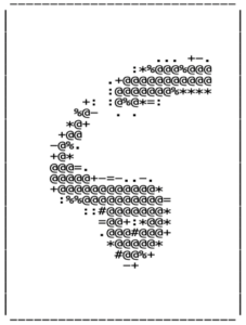
Confusion

So, let’s have a look on a few of the digits that the network typically confuses:

Digit:	Label:	Neural net:
	5	6
	5	3
	2	6

These are just a few examples. Several other border-cases are available too. It makes sense that the network find it quite hard to classify these and the reason ties back to what we discussed in the ending section of the first part in this series: some of these points in the 784D-space are simply too far away from their group of digits and possibly closer to some other group of points/digits. Or in natural language: They look more like some other digit than the one they are supposed to represent.

This is not to say that we don’t care about those hard cases. Quite the contrary. The world is a truly ambiguous place and machine learning needs to be able to handle ambiguity & nuances. You know, to be less machine-like (“Affirmative”) and more human (“No problemo”). But what I think this indicates is that the solution is not always in the data at hand. Quite often the context gives the clues needed for a human to correctly classify (or understand) something … such as a badly written digit. But that is another big and fascinating topic which falls outside this introduction.

Wrap up

This was the fifth and final part in this series. I learned a lot while writing this and I hope you did learn something by reading it.

Feel free to reach out. Feedback is welcome!

Good resources for further reading

These are the resources which I have found out to be better than most others. Please dive in if you want a slightly deeper understanding:

3 Blue 1 Browns fantastic videos on neural networks (4 episodes)
Michael Nielsens brilliant tutorial (several chapters)
Stanford course CS231n.
Explained.ai.

This article has also been published in the Medium-publication Towards Data Science. If you liked what you’ve just read please head over to the medium-article and give it a few Claps. It will help others finding it too. And of course I hope you spread the word in any other way you see fit. Thanks!

Footnotes:

One way to deal with this is to split the training data further so that we reserve a subset for hyper parameter tuning (a subset that we do not train the network on) and keep the test-data unseen for as long as possible.

Machine Learning

Tobias Hill