In this article we will build upon the basic neural network presented in part 3. We will add a few gems which will improve the network. Small changes with great impact. The concepts we will meet, such as Initialization, Mini batches, Parallelization, Optimizers and Regularization are no doubt things you would run into quickly when learning about neural networks. This article will give a guided tour-by-example.

This is the forth part in a series of articles:

• Part 1 – Foundation.
• Part 2 – Gradient descent and backpropagation.
• Part 3 – Implementation in Java.
• Part 4 – Better, faster, stronger.  (This article)
• Part 5 – Training the network to read handwritten digits.
• Extra 1 – Data augmentation.
• Extra 2 – A MNIST playground.

Initialization

Until now we have seen how weights and biases can be automatically adjusted via backpropagation to let the network improve. So what is a good starting value for these parameters?

Generally you are quite fine just to randomize the parameters between -0.5 and 0.5 with a mean of 0.

However, on deep networks, research has shown that we can get improved convergence if we let the values for the weights inversely depend on the number of neurons in the connected layer (or sometimes two connected layers). In other words: Many neurons ⇒ init weights closer to 0. Fewer neurons ⇒ higher variance can be allowed. You can read more about why here and here.

I have implemented a few of the more popular ones and made it possible to inject it as a strategy when creating the neural network:

The implemented strategies for initialization are: XavierNormal, XavierUniform, LeCunNormal, LeCunUniform, HeNormal, HeUniform and Random. You can also specify the weights for a layer explicitly by providing the weight matrix when the layer is being created.

Batching

In the last article we did briefly touch on the fact that we can feed samples through the network for as long  as we wish and then, at our own discretion, chose when to update the weights. The separation in the api between the evaluate()-method (which gathers learning/impressions) and the updateFromLearning()-method (which let that learning sink in) is there to allow exactly that. It leaves it open to the user of the API which of the following strategies to use:

Stochastic Gradient Descent

In Stochastic Gradient Descent we update the weights and biases after every evaluation. Remember from part 2 that the cost function is dependent on the input and the expectation: \(C = C(W, b, S_σ, x, exp)\). As a consequence the cost landscape will look slightly different for every sample and the negative gradient will point in the direction of steepest descent in that per-sample-unique landscape.

Now, let’s assume we have the total cost landscape which would be the averaged cost function for the entire dataset. All samples. Within that a Stochastic Gradient Descent would look like a chaotic walk.

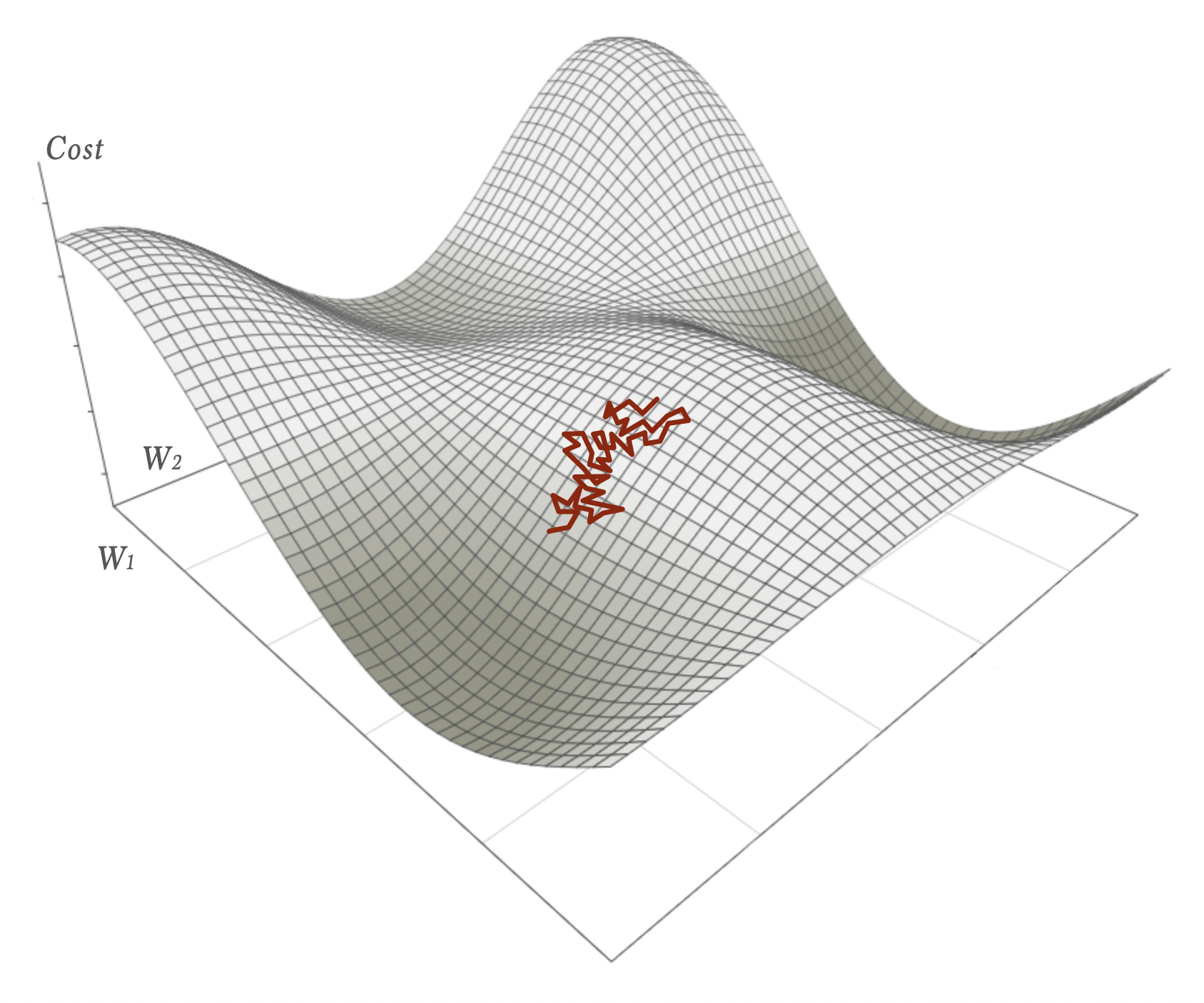
As long as the learning rate is reasonably small that walk would on average nevertheless descends towards a local minimum.

The problem is that SGD is hard to parallelize efficiently. Each update of the weights has to be part of the next calculation.

Batch Gradient Descent

The opposite of Stochastic Gradient Descent is the Batch Gradient Descent (or sometimes simply Gradient Descent). In this strategy all training data is evaluated before an update to the weights is made. The average gradient for all samples is calculated. This will converge towards a local minimum as carefully calculated small descending steps. The drawback is that the feedback loop might be very long for big datasets.

Mini-Batch Gradient Descent

Mini-batch gradient descent is a compromise between SGD and BGD – batches of N samples are run through the network before the weights are updated. Typically N is between 16 to 256. This way we get something that is quite stable in its descent (although not optimal):

• Compared to batch gradient descent we get faster feedback and can operate with manageable datasets.
• Compared to stochastic gradient descent we can run the whole batch in parallel using all of the cores on the CPU, GPU or the TPU. The best of two worlds.

Parallelizing

Only some minor changes had to be made to the code base  to allow parallel execution of the evaluation()-method. As always … state is the enemy of parallelization. In the feed forward phase the only state to treat with caution is the fact that the out-value from each neuron is stored per neuron. Competing threads would surely overwrite this data before it had been used in backpropagation.

By using thread confinement this could be handled.

Also the part where the deltas for the weights and biases are accumulated and finally applied had to be synchronized:

With that in place it is perfectly fine to use as many cores as desired (or available) when processing training data.

A typical way to parallelize mini batch execution on the neural net looks like this:

Especially note the construct for spreading the processing of all samples within the batch as a parallel stream in line 2.

That’s all needed.

Best of all: The speedup is significant¹.

One thing to keep in mind here is that spreading the execution this way (running a batch over several parallel threads) adds entropy to the calculation that is sometimes not wanted. To illustrate: when the error-deltas are summed in the addDeltaWeightsAndBiases-method they may be added in slightly different order every time you run. Although all contributing terms from the batch are the same the changed order they are summed may give small small differences which over time and in large neural nets starts to show, resulting in non-reproducible runs. This is probably fine in this kind of playground neural network implementation … but if you want to do research you would have to approach parallelism in a different way  (typically making big matrices of the input batch and parallel all the matrix-multiplications of both feed forward and backpropagation on GPUs/TPUs).

Optimizers

In last article we touched on the fact that we made the actual update of the weights and biases pluggable as a strategy. The reason is that there are other ways to do it than the basic gradient descent.

Remember, this:

$$W^+ = W -\eta\nabla C\tag{eq 1}\label{eq 1}$$

Which in code looks like:

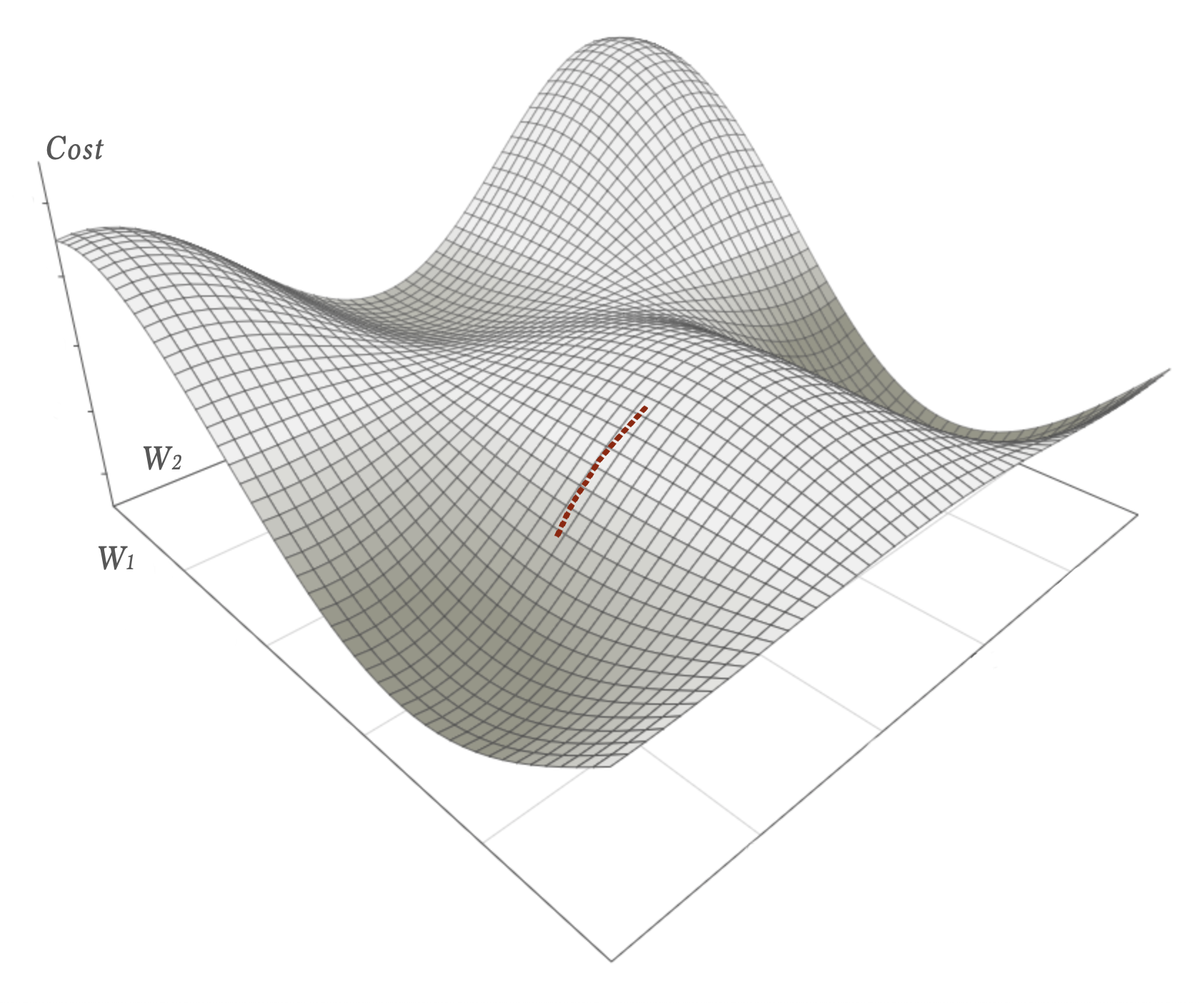
Although striving downhill the SGD (and its batched variants) suffers from the fact that the magnitude of the gradient is proportional to how steep the slope is at the point of evaluation. A flatter surface means a shorter length of the gradient … giving a smaller step. As a consequence it might get stuck on saddle points – for instance halfway down this path:

(as you can see there are better local minimas in several directions than getting stuck at that saddle point)

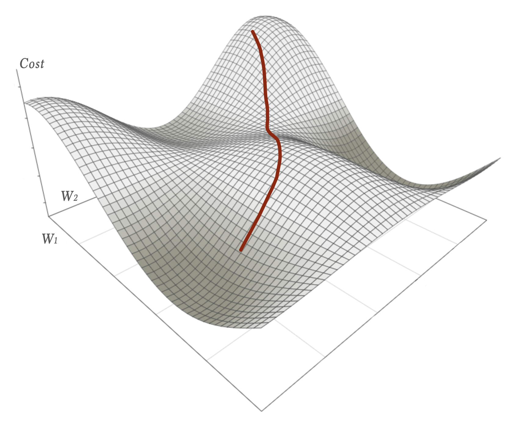
One way to better handle situations like this is to let the update of the weights not only depend on the calculated gradient but also the gradient calculated in last step. Somewhat like incorporating echos from previous calculations.

A physical analogy of this is to think of a marble with mass rolling down a hill. Such a marble might have enough momentum to keep enough of its speed to cover flatter parts or even climb up small hills – this way escaping the saddle point and continue towards better local minimas.

Not surprisingly one of the simplest Optimizers is called …

Momentum

In momentum we introduce another constant to tell how much echo we want from previous calculations. This factor, γ, is of called momentum. Equation 1 above now becomes:

$$
\begin{align}
v^+ &= \gamma v + \eta \nabla_w C\\[0.5em]
W^+ &= W – v^+
\end{align}
$$

As you can see the Momentum optimizer keeps the last delta as v and calculates a new v based on the previous one. Typically the γ could be in the range 0.7 – 0.9 which means that 70% – 90% of previous gradient calculations contributes to this new calculation.

In code it is configured as:

And applied in the Momentum optimizer like this:

This small change on how we update the weights often improves convergence.

We can do even better. Another simple yet powerful optimizer is the Nesterov accelerated gradient (NAG).

Nesterov accelerated gradient

The only difference from momentum is that we in NAG calculate the Cost at a position which has already incorporated the echo from last gradient calculation.

$$
\begin{align}
v^+ &= \gamma v + \eta \nabla_w C(W – \gamma v)\\[0.5em]
W^+ &= W – v^+
\end{align}
$$

From a programming perspective this is bad news. A nice property of the optimizers until now has been that they are only applied when the weights are updated. Here, all of a sudden, we need to incorporate the last gradient v already when calculating the cost function. Of course we could extend the idea of what an Optimizer is and allow it to also augment weight lookups for instance. That would not be coherent though since all other Optimizers (that I know of) only focus on the update.

With a small trick we can work around that problem. By introducing another variable x = W – γv we can rewrite the equations in terms of x. Specifically this introduction means that the problematic cost function would only be dependent on x and no historic v-value². After rewriting it we can rename x back to w again to make it look more like something we recognise. The equation becomes:

$$
\begin{align}
v^+ &= \gamma v – \eta \nabla_w C\\[0.5em]
W^+ &= W – \gamma v + (1 +\gamma) v^+
\end{align}
$$

Much better. Now the Nesterov optimizer can be applied only at update time:

To read more about how and why NAG often works better than Momentum please have a look here and here.

There are of course a lot of other fancy Optimizers that could have been implemented too. A few of them often perform better than NAG but at the cost of added complexity. In terms of improved convergence per lines of code NAG strikes a sweet spot.

Regularization

When I just had finished writing the first version of the neural network code I was eager to test it. I promptly downloaded the MNIST dataset and started playing around. Almost right off the bat I was up to quite remarkable figures in terms of accuracy. Comparing to what others had reached on equivalent network designs my was better – way better. This of course made me suspicious.

Then it struck me. I had compared my stats on the training dataset with their stats on the test dataset. I had trained my network in an infinite loop (almost) on the training data and never even loaded the test dataset. And when I did I got a shock. My network was totally crap on unseen data even though it was close to demigod on the training dataset. I had just swallowed the bitter pill of overfitting.

Overfitting

When you train your network too aggressively you might end up in a situation where your network has learned (almost memorised) the training data but as a side effect also lost the general broad strokes of what the training data represents. This can be seen by plotting the networks accuracy on the training data vs the test data during training of the network. Typically you will notice that the accuracy on the training data continues to increase while the accuracy on the test data initially increases after which it flattens out and then starts decreasing again.

This is when you’ve gone to far.

One observation here is that we need to be able to detect when this happens and stop training at that point. This is often referred to as Early stopping and something I will get back to in the last article in this series, Part 5 – Training the network to read handwritten digits.

But there are a few other ways to reduce the risk of overfitting too. I will wrap up this article by presenting a simple, but powerful approach.

L2 Regularization

In L2 regularization we we try to avoid that individual weights in the network get too big (or to be more precise: too far away from zero). The idea is that instead of letting a few weights have a very strong influence over the output we instead prefer that lot of weights interact, each and everyone with a moderate contribution. Based on the discussion in Part 1 – Foundation it does not seem too far fetched that several smaller weights (when compared to fewer bigger) will give a smoother and less sharp/peaky separation of the input data. Moreover, it seems reasonable that a smoother separation will retain general characteristics of the input data and conversely: a sharp and peaky ditto would be able to very precisely cut out the specific characteristics of the input data.

So how do we avoid that individual weights in the network get too big?

In L2 regularization this is accomplished by adding another cost-term to the cost function:

$$
\begin{eqnarray}
C = C_0 +\underbrace{\frac{\lambda}{2}\sum_w w^2}_{\text{new cost term}}
\end{eqnarray}
$$

As you can see big weights will contribute to a higher cost since they are squared in that additional cost sum. Smaller weights will not matter much at all.

The λ factor will tell how much L2 regularization we want. Setting it to zero will cancel the L2 effect altogether.  Setting it to, say 0.5, will let the L2 regularization be a substantial part of the total cost of the network. In practice you will have to find best possible λ given your network layout and your data.

Quite frankly we do not care much about the cost as a specific scalar value. We are more interested in what happens when we train the network via gradient descend. Let’s see what happens with the gradient calculation of this new cost function for a specific weight k.

$$
\begin{align}
\frac{\partial C}{\partial w_k} &=\frac{\partial C_0}{\partial w_k} +\frac{\partial}{\partial w_k}\frac{\lambda}{2}\sum_w w^2\\
&=\frac{\partial C_0}{\partial w_k} + \lambda w_k
\end{align}\tag{eq 2}\label{eq 2}
$$

As you can see we only get an additional term λw_k to subtract from the weight w_k in each update.

Sometimes you’ll see that the number of samples, n, and the learning-rate, η, is part of the update term – i.e. \(\frac{\eta\lambda}{n}w_k\). I see no reason to do so since \(\frac{\eta\lambda}{n}\) is just another constant.

In code, L2 regularization can be configured as:

And is applied at update-time in this way:

This minor change makes the neural network implementation a lot easier to control when it comes to overfitting.

So, that’s a wrap for this article. Several small gems have been presented in both theory and practice … all of which, with only a few lines of code, makes the neural network better, faster and stronger.

In the next article, which will be the final one in this series, we will see how well the network performs on a classical dataset – Mnist: Part 5 – Training the network to read handwritten digits.

Feedback is welcome!

This article has also been published in the Medium-publication Towards Data Science. If you liked what you’ve just read please head over to the medium-article and give it a few Claps. It will help others finding it too. And of course I hope you spread the word in any other way you see fit. Thanks!

Footnotes:

1. Of course not even close to the speedup you would get if you would push all matrix operations out to GPU:s for parallel calculation … but still: as a low hanging fruit this minor change is motivated.
2. At least not explicitly dependent. The -γv part would in fact still be used but now implicitly stored on all weights.