In this article you will see how the theories presented in previous two articles can be implemented in easy to understand java code. The full neural network implementation can be downloaded, inspected in detail, built upon and experimented with.
This is the third part in a series of articles:
- Part 1 – Foundation.
- Part 2 – Gradient descent and backpropagation.
- Part 3 – Implementation in Java. (This article)
- Part 4 – Better, faster, stronger.
- Part 5 – Training the network to read handwritten digits.
- Extra 1 – Data augmentation.
- Extra 2 – A MNIST playground.
I assume you have read both previous articles and have a fairly good understanding about the forward pass and the learning/training pass of a neural network.
This article will be quite different. It will show and describe it all in a few snippets of java code.
All my code – a fully working neural net implementation – can be found, examined & downloaded here.
Ambition
Normally when writing software I use a fair amount of open source – as a way to get good results faster and to be able to use fine abstractions someone else put a lot of thought into.
This time it is different though. My ambition is to show how a neural network works with a minimal requirement on your part in terms of knowing other open source libraries. If you manage to read Java 8 code you should be fine. It is all there in a few short and tidy files.
A consequence of this ambition is that I have not even imported a library for Linear Algebra. Instead two simple classes have been created with just the operations needed – meet the usual suspects: the Vec and the Matrix class. These are both very ordinary implementations and contain the typical arithmetic operations additions, subtractions, multiplications and dot-product.
The fine thing about vectors and matrices is that they often can be used to make code expressive and tidy. Typically when you are faced with doing operation on every element from one set with every other on the other set, like for instance weighted sums over a set of inputs, there is a good chance you can arrange your data in vectors and/or matrices and get a very compact and expressive code. A neural network is no exceptions to this1.
I too have collapsed the calculations as much as possible by using objects of types Vec and Matrix. The result is neat and tidy and not far from mathematical expressions. No for-loops in for-loops are blurring the top view. However, when inspecting the code I encourage you to make sure that any neat looking call on objects of type Vec or Matrix in fact results in exactly the series of arithmetic operations which were defined in part 1 and part 2.
Two operations on the Vec class is not as common as the typical ones I mentioned above. Those are:
- The outer product (Vec.outerProduct()) which is the element wise multiplication of a column vector and row vector resulting in a matrix.
- The Hadamard product (Vec.elementProduct()) which simply is the element wise multiplication of two vectors (both being column or row vectors) resulting in a new vector.
Overview
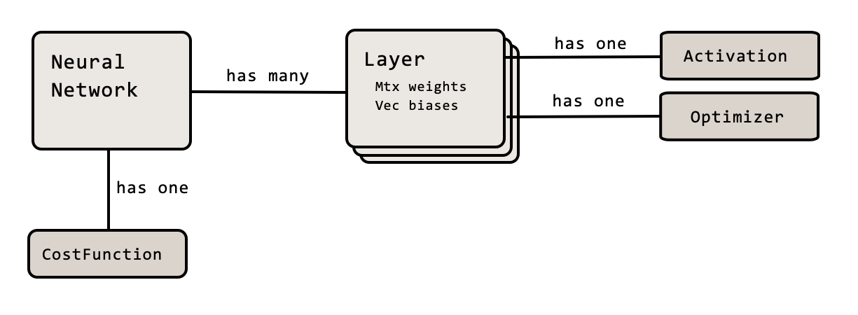
A typical NeuralNetwork has many Layers. Each Layer can be of any size and contains the weights between the preceding layer and itself as well as the biases. Each layer is also configured with an Activation and an Optimizer (more on what that is later).
Whenever designing something that should be highly configurable the builder pattern is a good choice2. This gives us a very straightforward and readable way to define and create neural networks:
|
1 2 3 4 5 6 7 8 |
NeuralNetwork network = new NeuralNetwork.Builder(30) // input to network is of size 30 .addLayer(new Layer(20, ReLU)) .addLayer(new Layer(16, Sigmoid)) .addLayer(new Layer(8, Sigmoid)) .setCostFunction(new CostFunction.Quadratic()) .setOptimizer(new GradientDescent(0.01)) .create(); |
To use such a network you typically either feed a single input vector to it or you also add an expected result in the call to evaluate()-method. When doing the latter the network will observe the difference between the actual output and the expected and store an impression of this. In other words, it will backpropagate the error. For good reasons (which I will get back to in the next article) the network does not immediately update its weights and biases. To do so – i.e. let any impressions “sink in” – a call to updateFromLearning() has to be made.
For example:
|
1 2 3 4 5 6 7 8 9 10 11 12 13 |
// Evaluate without learning Vec in1 = new Vec(0.1, 0.7); Result out1 = network.evaluate(in1); // Evaluate with learning (i.e. an expected outcome is provided) Vec exp1 = new Vec(0.3, -0.2); Result out2 = network.evaluate(in1, exp1); // Let the observation "sink in" network.updateFromLearning(); // ... at this point we have a better network and the result from this call would be improved out2 = network.evaluate(i1, exp1); |
Feed forward
Let’s dive into the feed forward pass – the call to evaluate(). Please note in the marked lines below that the input data is passed through layer by layer:
|
1 2 3 4 5 6 7 8 9 10 11 12 13 14 15 16 17 18 19 |
/** * Evaluates an input vector, returning the networks output. * If <code>expected</code> is specified the result will contain * a cost and the network will gather some learning from this * operation. */ public Result evaluate(Vec input, Vec expected) { Vec signal = input; for (Layer layer : layers) signal = layer.evaluate(signal); if (expected != null) { learnFrom(expected); double cost = costFunction.getTotal(expected, signal); return new Result(signal, cost); } return new Result(signal); } |
Within the layer the input vector is multiplied with the weights and then the biases is added. That is in turn used as input to the activation function. See the marked line. The layer also stores the output vector since it is used in the backpropagation.
|
1 2 3 4 5 6 7 8 9 10 11 12 13 14 |
/** * Feed the in-vector, i, through this layer. * Stores a copy of the out vector. * @param i The input vector * @return The out vector o (i.e. the result of o = iW + b) */ public Vec evaluate(Vec i) { if (!hasPrecedingLayer()) { out.set(i); // No calculation i input layer, just store data } else { out.set(activation.fn(i.mul(weights).add(bias))); } return out.get(); } |
(The reason there are get and and set operation on the out variable I will get back to in next article. For now just think of it as a variable of type Vec)
Activation functions
The code contains a few predefined activation functions. Each of these contain both the actual activation function, σ, as well as the derivative, σ’.
|
1 2 3 4 5 6 7 8 9 10 11 12 13 14 15 16 17 18 19 20 21 22 23 24 25 26 27 28 29 30 31 32 33 34 35 36 37 38 39 40 41 |
// -------------------------------------------------------------------------- // --- A few predefined ones ------------------------------------------------ // -------------------------------------------------------------------------- // The simple properties of most activation functions as stated above makes // it easy to create the majority of them by just providing lambdas for // fn and the diff dfn. public static Activation ReLU = new Activation( "ReLU", x -> x <= 0 ? 0 : x, // fn x -> x <= 0 ? 0 : 1 // dFn ); public static Activation Leaky_ReLU = new Activation( "Leaky_ReLU", x -> x <= 0 ? 0.01 * x : x, // fn x -> x <= 0 ? 0.01 : 1 // dFn ); public static Activation Sigmoid = new Activation( "Sigmoid", Activation::sigmoidFn, // fn x -> sigmoidFn(x) * (1.0 - sigmoidFn(x)) // dFn ); public static Activation Softplus = new Activation( "Softplus", x -> log(1.0 + exp(x)), // fn Activation::sigmoidFn // dFn ); public static Activation Identity = new Activation( "Identity", x -> x, // fn x -> 1 // dFn ); private static double sigmoidFn(double x) { return 1.0 / (1.0 + exp(-x)); } |
Cost functions
Also there are a few cost functions included. The Quadratic looks like this:
|
1 2 3 4 5 6 7 8 9 10 11 12 13 14 15 16 17 18 19 20 |
/** * Cost function: Quadratic, C = ∑(y−exp)^2 */ class Quadratic implements CostFunction { @Override public String getName() { return "Quadratic"; } @Override public double getTotal(Vec expected, Vec actual) { Vec diff = actual.sub(expected); return diff.dot(diff); } @Override public Vec getDerivative(Vec expected, Vec actual) { return actual.sub(expected).mul(2); } } |
A cost function has one method for calculating the total cost (as a scalar) but also the important differentiation of the cost function to be used in the …
Backpropagation
As I mentioned above: if an expected outcome is passed to the evaluate function the network will learn from it. See the marked lines.
|
1 2 3 4 5 6 7 8 9 10 11 12 13 14 15 16 17 18 19 |
/** * Evaluates an input vector, returning the networks output. * If <code>expected</code> is specified the result will contain * a cost and the network will gather some learning from this * operation. */ public Result evaluate(Vec input, Vec expected) { Vec signal = input; for (Layer layer : layers) signal = layer.evaluate(signal); if (expected != null) { learnFrom(expected); double cost = costFunction.getTotal(expected, signal); return new Result(signal, cost); } return new Result(signal); } |
In the learnFrom()-method the actual backpropagation happens. Here you should be able to follow the steps from part 2 in detail in code. It is somewhat soothing too see that the rather lengthy mathematical expressions from part 2 just boils down to this:
|
1 2 3 4 5 6 7 8 9 10 11 12 13 14 15 16 17 18 19 20 21 22 23 24 25 26 27 28 29 |
/** * Will gather some learning based on the <code>expected</code> vector * and how that differs to the actual output from the network. This * difference (or error) is backpropagated through the net. To make * it possible to use mini batches the learning is not immediately * realized - i.e. <code>learnFrom</code> does not alter any weights. * Use <code>updateFromLearning()</code> to do that. */ private void learnFrom(Vec expected) { Layer layer = getLastLayer(); // The error is initially the derivative of cost-function. Vec dCdO = costFunction.getDerivative(expected, layer.getOut()); // iterate backwards through the layers do { Vec dCdI = layer.getActivation().dCdI(layer.getOut(), dCdO); Matrix dCdW = dCdI.outerProduct(layer.getPrecedingLayer().getOut()); // Store the deltas for weights and biases layer.addDeltaWeightsAndBiases(dCdW, dCdI); // prepare error propagation and store for next iteration dCdO = layer.getWeights().multiply(dCdI); layer = layer.getPrecedingLayer(); } while (layer.hasPrecedingLayer()); // Stop when we are at input layer } |
Please note that the learning (the partial derivatives) in the backpropagation is stored per layer by a call to addDeltaWeightsAndBiases()-method.
Not until a call to updateFromLearning()-method has been made the weights and biases change:
|
1 2 3 4 5 6 7 8 9 10 |
/** * Let all gathered (but not yet realised) learning "sink in". * That is: Update the weights and biases based on the deltas * collected during evaluation & training. */ public void updateFromLearning() { for (Layer l : layers) if (l.hasPrecedingLayer()) // Skip input layer l.updateWeightsAndBias(); } |
The reason why this is designed as two separate steps is that it allows the network to observe a lot of samples and learn from these … and then only finally update the weights and biases as an average of all observations. This is in fact call Batch Gradient Descent or Mini Batch Gradient Descent. We will get back to these variants in the next article. For now you can as well call updateFromLearning after each call to evaluate (with expectations) to make the network improve after each sample. That, to update the network after each sample, is called Stochastic Gradient Descent.
This is what the updateWeightsAndBias()-method looks like. Notice that an average of all calculated changes to the weights and biases is fed into the two methods updateWeights() and updateBias() on the optimizer object.
|
1 2 3 4 5 6 7 8 9 10 11 12 13 14 15 |
public synchronized void updateWeightsAndBias() { if (deltaWeightsAdded > 0) { Matrix average_dW = deltaWeights.mul(1.0 / deltaWeightsAdded); optimizer.updateWeights(weights, average_dW); deltaWeights.map(a -> 0); // Clear deltaWeightsAdded = 0; } if (deltaBiasAdded > 0) { Vec average_bias = deltaBias.mul(1.0 / deltaBiasAdded); bias = optimizer.updateBias(bias, average_bias); deltaBias = deltaBias.map(a -> 0); // Clear deltaBiasAdded = 0; } } |
We have not really talked about the concept of optimizers yet. We have only said that the weights and biases are updated by subtracting the partial derivatives scaled with some small learning rate – i.e:
$$w^+=w – \eta \frac {\partial C}{\partial w}$$
And yes, that is a good way to do it and it is easy to understand. However, there are other ways. A few of these are a bit more complicated but offers faster convergence. The different strategies on how to update weights and biases is often referred to as Optimizers. We will see another way to do it in the next article. As a consequence it is reasonable to leave this as a pluggable strategy that the network can be configured to use.
For now we just use the simple GradientDescent strategy for updating our weights and biases:
|
1 2 3 4 5 6 7 8 9 10 11 12 13 14 15 16 17 18 19 20 21 |
/** * Updates Weights and biases based on a constant learning rate - i.e. W -= η * dC/dW */ public class GradientDescent implements Optimizer { private double learningRate; public GradientDescent(double learningRate) { this.learningRate = learningRate; } @Override public void updateWeights(Matrix weights, Matrix dCdW) { weights.sub(dCdW.mul(learningRate)); } @Override public Vec updateBias(Vec bias, Vec dCdB) { return bias.sub(dCdB.mul(learningRate)); } } |
And that’s pretty much it. With a few lines of code we have the possibility to configure a neural network, feed data trough it and make it learn how to classify unseen data. This will be shown in Part 5 -Training the network to read handwritten digits.
But first, let’s pimp this up a few notches. See you in Part 4 – Better, faster, stronger.
Feedback is welcome!
This article has also been published in the Medium-publication Towards Data Science. If you liked what you’ve just read please head over to the medium-article and give it a few Claps. It will help others finding it too. And of course I hope you spread the word in any other way you see fit. Thanks!
Also, check out my new word game Crosswise!
Footnotes:
- Quite the contrary: the reason it is possible to speed up learning immensely on GPUs and TPUs is the huge amount of vector and matrix operations within the feed forward and backpropagation.
- Most code examples I have found explaining how a neural network works has quite an awful design. Almost without exception they define the network with a number of badly named multidimensional arrays with constants defining their sizes. A very static design not at all inviting you to try out different network setups.
Shouldn’t it be e.g. x -> x * (1.0 – x) for the derivative of the sigmoid function because you put the output of the layer after already having applied the activation function as x? The same applies to the other activation functions. In the case of Leaky ReLU it does make no difference because this function keeps the sign and softmax is defined separately.