In this article you will learn how a neural network can be trained by using backpropagation and stochastic gradient descent. The theories will be described thoroughly and a detailed example calculation is included where both weights and biases are updated.
This is the second part in a series of articles:
- Part 1 – Foundation.
- Part 2 – Gradient descent and backpropagation. (This article)
- Part 3 – Implementation in Java.
- Part 4 – Better, faster, stronger.
- Part 5 – Training the network to read handwritten digits.
- Extra 1 – Data augmentation.
- Extra 2 – A MNIST playground.
I assume you have read the last article and that you have a good idea about how a neural network can transform data. If the last article required a good imagination (thinking about subspaces in multi-dimensions) this article on the other hand will be more demanding in terms of math. Brace yourself: Paper and pen. A silent room. Careful thought. A good nights sleep. Time, stamina and effort. It will sink in.
Supervised learning
In the last article we concluded that a neural network can be used as a highly adjustable vector function. We adjust that function by changing weights and the biases but it is hard to change these by hand. They are often just too many and even if they were fewer it would nevertheless be very hard to get good results by hand.
The fine thing is that we can let the network adjust this by itself by training the network. This can be done in different ways. Here I will describe something called supervised learning. In this kind of learning we have a dataset that has been labeled – i.e. we already have the expected output for every input in this dataset. This will be our training dataset. We also make sure that we have a labeled dataset that we never train the network on. This will be our test dataset and will be used to verify how good the trained network classifies unseen data.
When training our neural network we feed sample by sample from the training dataset through the network and for each of these we inspect the outcome. In particular we check how much the outcome differs from what we expected – i.e. the label. The difference between what we expected and what we got is called the Cost (sometimes this is called Error or Loss). The cost tells us how right or wrong our neural network was on a particular sample. This measure can then be used to adjust the network slightly so that it will be less wrong the next time this sample is feed trough the network.
There are several different cost functions that can be used (see this list for instance).
In this article I will use the quadratic cost function:
$$
C = \sum\limits_j \left(y_j – exp_j\right)^2
$$
(Sometimes this is also written with a constant 0.5 in front which will make it slightly cleaner when we differentiate it. We will stick to the version above.)
Returning to our example from part 1.
If we expected:
$$
exp = \begin{bmatrix}
1 \\
0.2 \\
\end{bmatrix}
$$
… and got …
$$
y = \begin{bmatrix}
0.712257432295742 \\
0.533097573871501 \\
\end{bmatrix}
$$
… the cost would be:
$$
\begin{align}
C & = (1 – 0.712257432295742)^2\\[0.8ex]
& + (0.2 – 0.533097573871501)^2\\[0.8ex]
& = 0.287742567704258^2\\[0.8ex]
& + (-0.333097573871501)^2\\[0.8ex]
& = 0.0827957852690395\\[0.8ex]
& + 0.11095399371908007\\[0.8ex]
& = 0.19374977898811957
\end{align}
$$
As the cost function is written above the size of the error explicitly depends on the network output and what value we expected. If we instead define the cost in terms of the inputed value (which of course is deterministically related to the output if we also consider all weights, biases and what activation functions were used) we could instead write \(C = C(y, exp) = C(W, b, S_σ, x, exp)\) – i.e. the cost is a function of the Weights, the biases, the set of activation functions, the input x, and the expectation.
The cost is just a scalar value for all this input. Since the function is continuous and differentiable (sometimes only piecewise differentiable. For example when ReLU-activations are used) we can imagine a continuous landscape of hills and valleys for the cost function. In higher dimensions this landscape is hard to visualize but with only two weights w1 and w2 it might look somewhat like this:
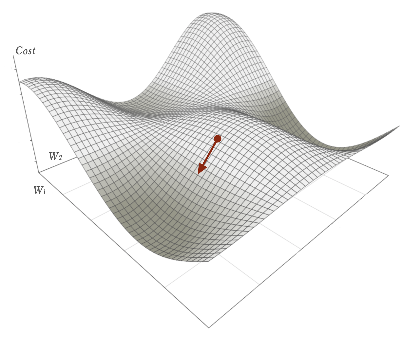
Suppose we got exactly the cost-value specified by the red dot in the image (based on just a w1 and w2 in that simplified case). Our aim now is to improve the neural network. If we could reduce the cost the neural network would be better at classifying our labeled data. Preferably we would like to find the global minimum of the cost-function within this landscape. In other words: the deepest valley of them all. Doing so is hard and there are no explicit methods for such a complex function that a neural network is. However, we can find a local minimum by using an iterative process called Gradient Descent. A local minimum might be sufficient for our needs and if not we can always adjust the network design in order to get a new cost-landscape to explore locally and iteratively.
Gradient Descent
From multivariable calculus we know that the gradient of a function, \(\nabla f\) at a specific point will be a vector tangential to the surface pointing in the direction where the function increases most rapidly. Conversely, the negative gradient \(-\nabla f\) will point in the direction where the function decreases most rapidly. This fact we can use to calculate new weights W+ from our current weights W:
$$
W^+ = W -\eta\nabla C\tag{eq 1}\label{eq 1}
$$
In the equation above \(\eta\) is just a small constant called learning-rate. This constant tells us how much of the gradient vector we will use to change our current set of weights into new ones. If chosen too small the weights will be adjusted too slowly and our convergence towards a local minimum will take long time. If set too high we might overshoot and miss (or get a bouncy non-convergent iterative behaviour).
All things in the equation above is just simple matrix arithmetics. The thing we need to take a closer look at is the gradient of the cost function with respect to the weights:
$$
\nabla C = \begin{bmatrix}
\frac{\partial C}{\partial w_1} \\
\frac{\partial C}{\partial w_2} \\
\vdots\\
\frac{\partial C}{\partial w_n} \\
\end{bmatrix}
$$
As you see we are for the time being not interested in the specific scalar cost value, C, but rather how much the Cost function changes when the weights changes (calculated one by one).
If we expand the neat vector form \(\eqref{eq 1}\) it looks like this:
$$
\begin{bmatrix}
w^+_1\\
w^+_2\\
\vdots\\
w^+_n\\
\end{bmatrix}
=
\begin{bmatrix}
w_1\\
w_2\\
\vdots\\
w_n\\
\end{bmatrix}
– \eta
\begin{bmatrix}
\frac{\partial C}{\partial w_1} \\
\frac{\partial C}{\partial w_2} \\
\vdots\\
\frac{\partial C}{\partial w_n} \\
\end{bmatrix}
$$
The fine thing about using the gradient is that it will adjust those weights that are in most need for a change more, and the weights in less need of change less. That is closely connected to the fact that the negative gradient vector points exactly in the direction of maximum descent. To see this please have a look once again at the simplified cost-function landscape image above and try to visualize a separation of the red gradient vector into to its component vectors along the axes.
The gradient descent idea works just as fine in N dimensions, although it is hard to visualize it. The gradient will still tell which components need to change more and which ones need to change less to reduce the function C.
So far I have just talked about weights. What about the biases? Well, the same reasoning is just as valid for them but instead we calculate (which is simpler):
$$\frac{\partial C}{\partial b}$$
Now it is time to see how we can calculate all these partial derivatives for both weights and biases. This will lead us into a more hairy territory so buckle up. To make sense of it all first we need a word on …
Notation
The rest of this article is notation intense. A lot of the symbols and letters you will see is just there as subscripted indexes to help us keep track on which layer and neuron I am referring to. Don’t let these indexes make the mathematical expressions become intimidating. The indexes are there to help and to make it more precise. Here is a short guide on how to read them:
- wL – a weight in the last layer.
- wH – a weight in a hidden layer.
- wk – a specific weight k.
- iL – input to a neuron in the last layer.
- iH – input to a neuron in a hidden layer.
- oL – output from a neuron in the last layer.
- oH – output from a neuron in a hidden layer.
- oLn – output from neuron n in the last layer.
- \({\partial x}\) – … all of the above is often prefixed with the partial derivative symbol. When that is the case think of it as an expression for how much x changes.
Also please pay attention to that the input to the neuron was called z in last article (which is quite common too) but has been changed to i here. The reason is that I find it easier to remember it as i for input and o for output.
Backpropagation
The easiest way to describe how to calculate the partial derivatives is to look at one specific single weight:
$$\frac{\partial C}{\partial w_k}$$
… i.e. how much does the total cost change when exactly that wk changes.
We will also see that there is a slight difference how to treat the partial derivative if that specific weight is connected to the last output layer or if it is connected to any of the preceding hidden layers.
Last layer
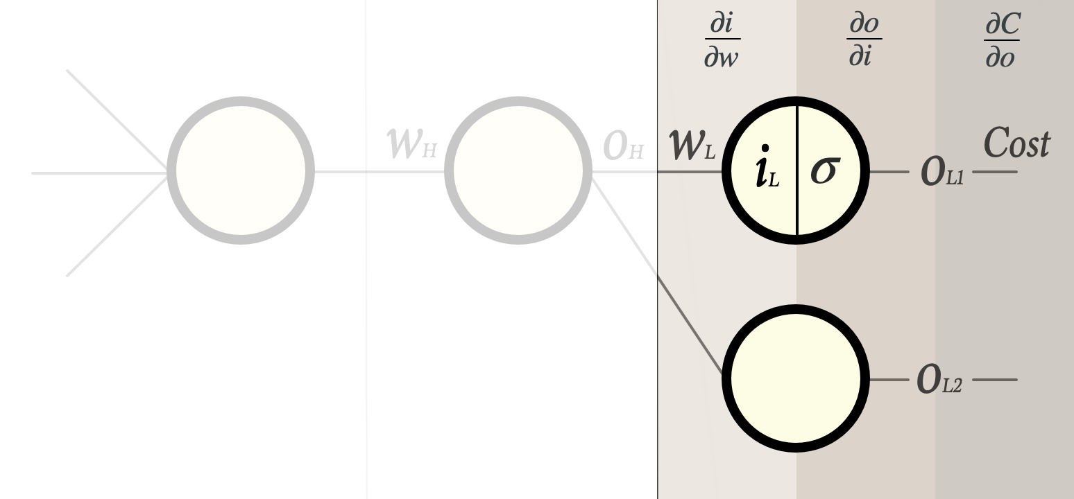
Now consider a single weight wL in the last layer:
Our task is to find:
$$\frac{\partial C}{\partial w_L}$$
As outlined in last article there are a few steps between the weight and the cost function:
- We multiply the weight with the output from preceding layer and add a bias. The result is the input iL to the neuron.
- This iL is then fed through the activation function σ, producing an output from the neuron oL1
- Finally this oL1 is used in the cost function.
It is fair to say that it is hard to calculate …
$$\frac{\partial C}{\partial w_L}$$
… just by looking at it. However, if we separate it into the three steps I just described things get a lot easier. Since the three steps are chained functions we could separate the derivative of it all by using the chain rule from calculus:
$$
\frac{\partial C}{\partial w_L} = \frac{\partial i_L}{\partial w_L}\frac{\partial o_{L1}}{\partial i_L}\frac{\partial C}{\partial o_{L1}}\tag{eq 2}\label{eq 2}
$$
As a matter of fact these three partial derivatives happens to be straightforward to calculate:
| $$\frac{\partial i_L}{\partial w_L}$$ | How much does the input value to the neuron change when wL changes? The input to the neuron is oHwL + b. The derivative of this with respect to wL is simply oH – the output from the previous layer. |
| $$\frac{\partial o_{L1}}{\partial i_L}$$ | How much does the output from the neuron change when the input changes? The only function transforming the input to output is the activation function – hence we just need the derivative of the activation function σ’.
|
| $$\frac{\partial C}{\partial o_{L1}}$$ | How much does the cost change when the output from the neuron changes? This is simply the derivative of the cost-function with respect to a specific out value.
In the case of the Quadratic cost function: (For this specific (nice) cost function the derivative of all others terms in that total cost sum is 0 since they do not depend on oL1) |
This means we have all three factors needed for calculating
$$\frac{\partial C}{\partial w_L}$$
In other words we now know how to update all weights in the last layer.
Let’s work our way backwards from here.
Hidden layers
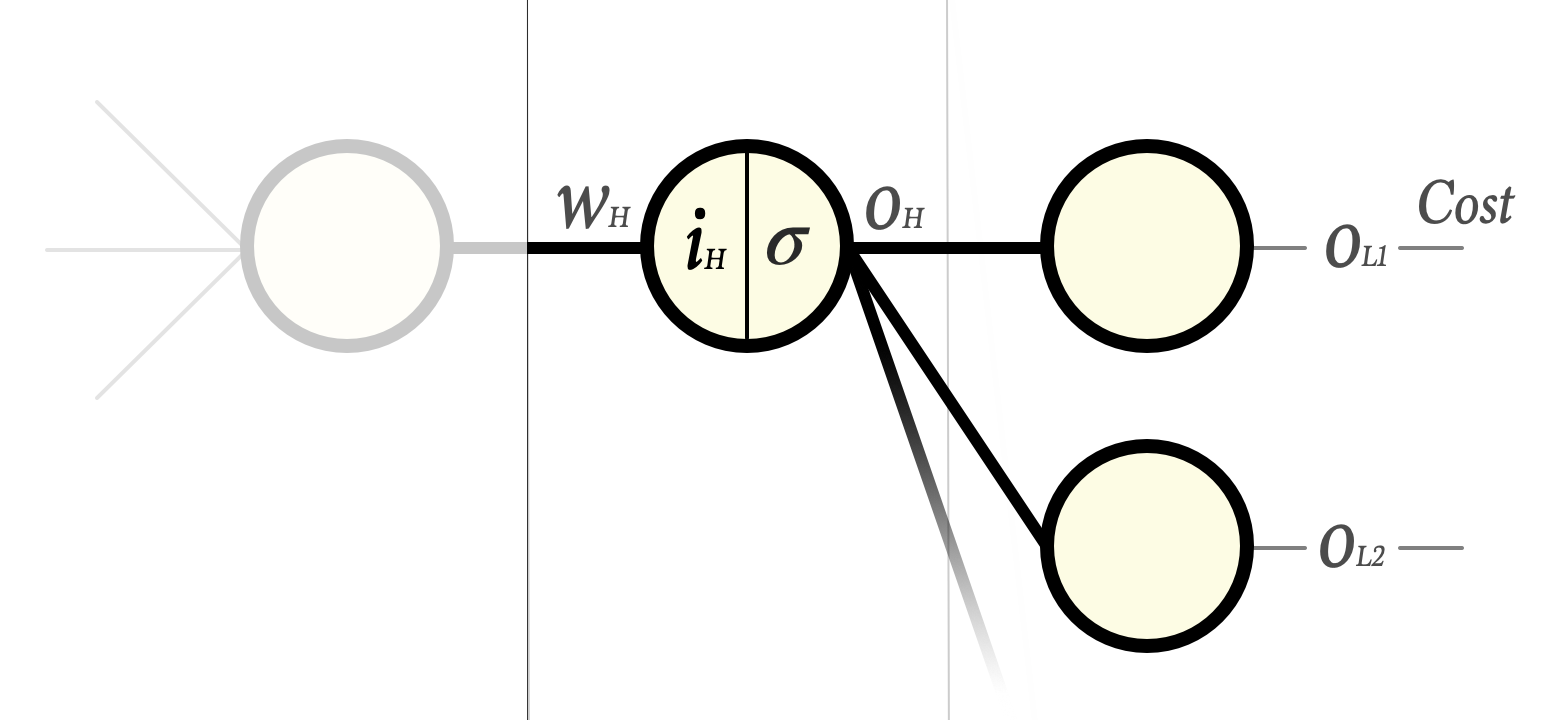
Now consider a single weight wH in the hidden layer before the last layer:
Our goal is to find
$$\frac{\partial C}{\partial w_H}$$
… i.e. how much a change in wH would change the total cost.
We proceed as we did in the last layer. The chain rule gives us:
$$
\frac{\partial C}{\partial w_H} = \frac{\partial i_H}{\partial w_H}\frac{\partial o_{H}}{\partial i_H}\frac{\partial C}{\partial o_{H}}
$$
The two first factors are the same as before and resolves to:
- the output from the preceding layer and …
- the derivative of the activation function respectively.
However, the factor …
$$\frac{\partial C}{\partial o_{H}}$$
… is a bit more tricky. The reason is that a change in oH obviously changes the input to all neurons in the last layer and as a consequence alters the cost function in a much broader sense as compared to when we just had to care about one output from a single last layer neuron (I have illustrated this by making the connections wider in the image above).
To resolve this we need to split the partial derivative of the total cost function into each and every contribution from the last layer.
$$
\frac{\partial C}{\partial o_{H}} = \frac{\partial C_{oL1}}{\partial o_{H}} + \frac{\partial C_{oL2}}{\partial o_{H}} + \cdots + \frac{\partial C_{oLn}}{\partial o_{H}}
$$
… where each term describes how much the Cost changes when oH changes, but only for that part of the signal that is routed via that specific output neuron.
Let’s inspect that single term for the first neuron. Again it will get a bit clearer if we separate it by using the chain rule:
$$
\frac{\partial C_{oL1}}{\partial o_{H}} = \frac{\partial i_{L1}}{\partial o_{H}} \frac{\partial C_{oL1}}{\partial i_{L1}}
$$
Let’s look at each of these:
| $$\frac{\partial i_{L1}}{\partial o_{H}}$$ | How much does the input to the last layer change when the output of the neuron in the current hidden layer changes?
The input to the last layer neuron is iL1 = oHwL + b. This time however please note that we are interested in the partial derivative of oH why the result simply is w. |
| $$\frac{\partial C_{oL1}}{\partial i_{L1}}$$ | How much does the cost change when the input to the last layer changes?
But hang on … doesn’t this look familiar? It should because this is exactly what we had a moment ago for this neuron when we calculated the weight adjustments of the last layer. In fact it is just the two last factors in chain \(\eqref{eq 2}\). This is a very important realisation and the magic part of backpropagation. |
Let’s pause for a moment and let it all sink in.
To summarize what we’ve just found out:
- To know how to update a specific weight in a hidden layer we take the partial derivative of the Cost in terms of that weight.
- By applying the chain rule we end up with three factors where two of those we already know how to calculate.
- The third factor in that chain is the weighted sum of a product of two factors we already calculated in the last layer.
- This means we can calculate all weights in this hidden layer the same way as we did in the last layer with the only difference that we use already calculated data from the previous layer instead of the derivative of the cost function.
From a computational viewpoint this very good news since we are only depending on calculations we just did (last layer only) and we do not have to traverse deeper than that. This is sometimes called dynamic programming which often is a radical way to speed up a an algorithm once the dynamic algorithm is found.
And since we only depend on generic calculations in the last layer (in particular we are not depending on the cost function) we can now proceed backwards layer by layer. No hidden layer is different from any other layer in terms of how we calculate the weight updates. We say that we let the cost (or error or loss) backpropagate. When we reach the first layer we are done. At that point we have partial derivatives for all weights in the equation \(\eqref{eq 1}\) and are ready to make our gradient descent step downhill in the cost function landscape.
And you know what: that’s it.
Hey WAIT … the Biases!?
Ok, I hear you. Actually they follow the same pattern. The only difference is that the first term in the derivative chain of both the last layer and the hidden layer expressions would be:
$$\frac{\partial i}{\partial b}$$
… instead of
$$\frac{\partial i}{\partial w}$$
Since the input to the neuron is oHwL+b the partial derivative of that with respect to b simply is 1. So where we in the weight case multiplied the chain with the output from last layer we simply ignore the output in the bias case and multiply with one.
All other calculations are identical. You can think of the biases as a simpler sub-case to the weight calculations. The fact that a change in the biases does not depend on the output from previous neuron actually makes sense. The biases are added “from the side” regardless of the data coming on the wire to the neuron.
An example
From my quite recent descent into backpropagation-land I can imagine that the reading above can be quite something to digest. Don’t be paralyzed. In practice it is quite straightforward and probably all things get clearer and easier to understand if illustrated with an example.
Let’s build on the example from Part 1 – Foundation:
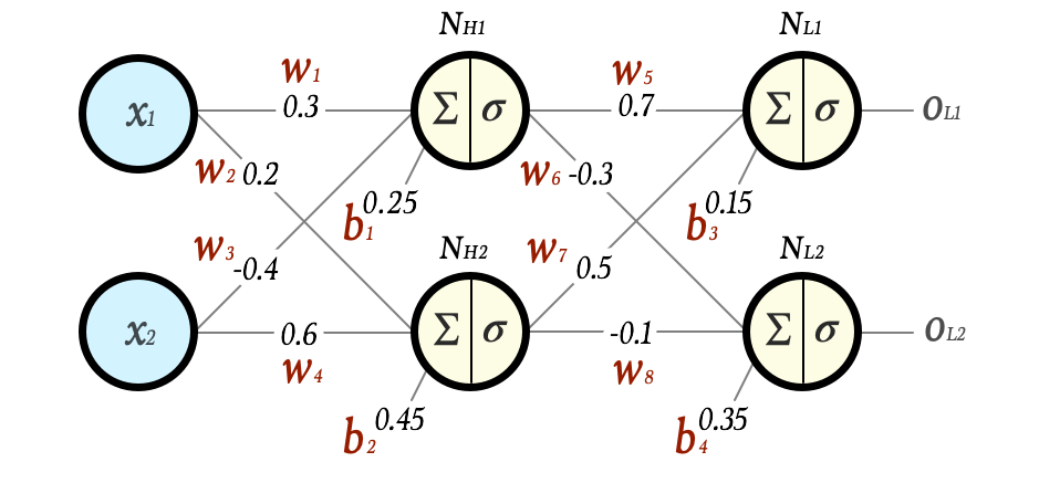
Let us start with w5:
$$
\begin{align}
\frac{\partial C}{\partial w_5} & = \frac{\partial i_L}{\partial w_5}\frac{\partial o_{L1}}{\partial i_L}\frac{\partial C}{\partial o_{L1}} \\[1.2ex]
& = O_{h1}\cdot \sigma'(O_{L1}) \cdot 2 (O_{L1} – exp_{L1})\\[1.2ex]
\end{align}
$$
By picking data from the forward pass in part 1 and by using data from the example cost calculation above we will calculate factor by factor. Also let’s assume that we have a learning rate of η = 0.1 for this example.
$$
\begin{align}
O_{h1} & = 0.41338242108267 \\[0.8ex]
\\[0.8ex]
\sigma'(O_{L1}) & = \sigma(I_{L1})(1 -\sigma(I_{L1})) \\[0.8ex]
& = 0.220793265944315 \\[0.8ex]
\\[0.8ex]
2 (O_{L1} – exp_{L1}) & = 2 \cdot (0.712257432295742 – 1)\\[0.8ex]
& = 2\cdot -0.2877425677042583\\[0.8ex]
&= -0.5754851354085166\\[0.8ex]
\\[0.8ex]
\frac{\partial C}{\partial w_5} & =0.41338242108267\\[0.1ex]
& \cdot 0.220793265944315\\[0.1ex]
& \cdot-0.57548513540851\\[0.1ex]
& = -0.052525710835624\tag{eq 3}\label{eq 3}\\[0.8ex]
\\[0.8ex]
\boldsymbol{w^+_5} & = w_5 – \eta \cdot \frac{\partial C}{\partial w_5} \\[0.8ex]
&= 0.7 – 0.1(-0.052525710835624) \\[0.8ex]
& = 0.70525257108356 \\[0.8ex]
\end{align}
$$
Likewise we can calculate all other parameters in the last layer:
$$
\begin{align}
\boldsymbol{w^+_6} & = -0.3064179482696209 \\[0.8ex]
\boldsymbol{w^+_7} & = 0.5118678465030685 \\[0.8ex]
\boldsymbol{w^+_8} & = -0.11450094129460808 \\[0.8ex]
\boldsymbol{b^+_3} & = 0.1627063242549253 \\[0.8ex]
\boldsymbol{b^+_4} & = 0.33447454961240974 \\[0.8ex]
\end{align}
$$
Now we move one layer backwards and focuses on w1:
$$
\begin{align}
\frac{\partial C}{\partial w_1} & = \frac{\partial i_{H1}}{\partial w_1} \frac{\partial o_{H1}}{\partial i_{H1}}\cdot \left(\sum\limits_j{\frac{\partial C_{oLj}}{\partial o_{H1}}}\right)\\[0.8ex]
& = \frac{\partial i_H}{\partial w_H}\frac{\partial o_{H1}}{\partial i_H}\cdot \left(\frac{\partial C_{oL1}}{\partial o_{H1}} + \frac{\partial C_{oL2}}{\partial o_{H1}}\right) \\[0.8ex]
& = \frac{\partial i_H}{\partial w_H}\frac{\partial o_{H1}}{\partial i_H}\cdot
\left(
\frac{\partial i_{L1}}{\partial o_{H}} \frac{\partial C_{oL1}}{\partial i_{L1}} +
\frac{\partial i_{L2}}{\partial o_{H}} \frac{\partial C_{oL2}}{\partial i_{L2}}
\right)
\\[1.2ex]
& = x_{1}\cdot \sigma'(O_{H1}) \cdot
\left(
w_5\frac{\partial C_{oL1}}{\partial i_{L1}} +
w_6\frac{\partial C_{oL2}}{\partial i_{L2}}
\right)
\\[1.2ex]
\end{align}
$$
Once again, by picking data from the forward pass in part 1 and by using data from above this is straightforward to calculate factor by factor.
$$
\begin{align}
x_1 & = 2 \\[0.1ex]
\\[0.1ex]
\sigma'(O_{H1}) & = \sigma(I_{H1})(1 -\sigma(I_{H1})) \\[0.8ex]
& = 0.23961666676227233 \\[0.8ex]
\\[0.8ex]
w_5 &= 0.7\\[0.8ex]
w_6 &= -0.3\\[0.8ex]
\end{align}
$$
From calculations in last layer:
$$
\begin{align}
\frac{\partial C_{oL1}} {\partial i_{L1}} &= 0.220793… \cdot -0.575485… \text{ (from }\eqref{eq 3}\text{)}\\[0.1ex]
&= -0.127063242549253\\[0.1ex]
\\[0.8ex]
\frac{\partial C_{oL2}} {\partial i_{L2}} &= 0.15525450387590206\\[0.1ex]
& \text{ (calculated likewise, not shown)}\\[0.8ex]
\\[0.8ex]
\end{align}
$$
Now we have it all and can finally find w1:
$$
\begin{align}
\frac{\partial C}{\partial w_1} & = 2 \cdot 0.239616666762272 \\[0.8ex]
& \cdot (0.7 \cdot −0.127063… + (-0.3) \cdot 0.155254…)\\[0.8ex]
& = -0.064945998937865\\[0.8ex]
\\[0.8ex]
\boldsymbol{w^+_1} & = w_1 – \eta \cdot \frac{\partial C}{\partial w_1} \\[0.8ex]
&= 0.3 – 0.1(-0.064945998937865) \\[0.8ex]
& = 0.3064945998937866 \\[0.8ex]
\end{align}
$$
In the same manner we can calculate all other parameters in the hidden layer:
$$
\begin{align}
\boldsymbol{w^+_2} & = 0.20320220163143507 \\[0.8ex]
\boldsymbol{w^+_3} & = -0.39025810015932016\\[0.8ex]
\boldsymbol{w^+_4} & = 0.6048033024471525\\[0.8ex]
\boldsymbol{b^+_1} & = 0.25324729994689327\\[0.8ex]
\boldsymbol{b^+_2} & = 0.4516011008157175 \\[0.8ex]
\end{align}
$$
That’s it. We have successfully updated the weights and biases in the whole network!
Sanity check
Let us verify that the network now behaves slightly better on the input
x = [2, 3].
First time we fed that vector through the network we got the output
y = [0.712257432295742 0.533097573871501]
… and a cost of 0.19374977898811957.
Now, after we have updated the weights we get the output
y = [0.719269360605435 0.524309343003261]
… and a cost of 0.1839862418540884.
Please note that both components have moved slightly towards what we expected, [1, 0.2], and that the total cost for the network is now lower.
Repeated training will make it even better!
Next article shows how this looks in java code. When you feel ready for it, please dive in: Part 3 – Implementation in Java.
Feedback is welcome!
This article has also been published in the Medium-publication Towards Data Science. If you liked what you’ve just read please head over to the medium-article and give it a few Claps. It will help others finding it too. And of course I hope you spread the word in any other way you see fit. Thanks!
Also, check out my new word game Crosswise!
A beautiful numerical illustration of how a continuous application of the chain rule and partial derivatives can yield almost magical results in finding local minimums! My question would be what if the local minimum is not the global minimum?
Hi Chandru,
It is almost never the global minimum. The lowest valley of them all is very hard to find in the multidimensional cost-function-landscape. We have no analytical nor efficient numerical methods for that. However, local minimas often suffice.
good evening Tobias
Thanks you very much for your tutorial but in the explanation of the hidden layer weight calculating the value -0.0641679049644533 seems to be wrong. The specified formula returns the value -0.054231533731954. Can you clarify if it is a calculation error or update the formula used? Thanks a lot Giulio
Good spotting. I’ll fix that.
Actually. While going through the calculations once again I also found that I was taking a shortcut when doing the derivative of the sigmoid function. That shortcut would have been possible when there is no bias on the neuron … which is not the case in the example. Hence I had to redo the calculations all the way – i.e. more than one number have changed.
If you find anything else that looks odd, please feedback it. Thanks!